Exploritory Hypothesis:

Can the data that I’ve collected through one journal provide me with deeper personal insight into who I am? My mood fluctations? The probability of fluctuations?

Dataset and measurement explainations:

Each time I made a journal entry I recorded my mood for the day at the time using a 0-10 scale. Zero being the worst and 10 being the best. In February 2008 I experimented with a line and tick mark as well as floating point integers. These have all been rounded or numerically approximated.

Mood analysis conducted over 168 entries within 14 months, Feb2008 – Apr2009.

Begin R Code:

library(zoo) #For non-fixed interval data
library (psych) #For descriptive statistics
library (ggplot2) #For better looking histograms

###Data manually entered right out of my journal from dated entries during the month.
month <- as.yearmon (2008 + seq(1,15)/12) 


feb08 <- c(3,6,7,7,8,8,8,10,9,0,0,5,7)
mar08 <- c(5,0,7,7,10,10,7,6,6,5,6,4,6)
apr08 <- c(5,7)
may08 <- c(7)
jun08 <- c(8,6)
jul08 <- c(6,7,6,6,6,7,6,5,7,6,4,5)
aug08 <- c(3,8,6,6,6,6,5)
sept08 <- c(6,7,9,5,7,8,7)
oct08 <- c(3,6,7,6,8,8,5,7,8,5,8,5,7,10,6,6)
nov08 <- c(5,6,7,7,7,7,5,7,7)
dec08 <- c(7,6,6,10,6,7,6,6,6,5,4,5,4,6,6,6)
jan09 <- c(5,7,6,7,5,6,5,7,3,7,6,7,8,7,6,6,7,5,5,4,6,4,2)
feb09 <- c(7,7,8,7,8,6,7,7,6,7,5,8,6,7,6,7,8,7)
mar09 <- c(3,5,7,6,4,6,5,6,2,3,6,6,5,5,5,5,6,7,6,5)
apr09 <- c(6,6,7,8,6,7,9,7,6)

###Now I'm ready to build the vector mood
mood <- c(feb08, mar08, apr08, may08, jun08, jul08, aug08, sept08, oct08, nov08, 
dec08, jan09, feb09, mar09, apr09)

describe(mood)

##   var   n mean   sd median trimmed  mad min max range skew kurtosis   se
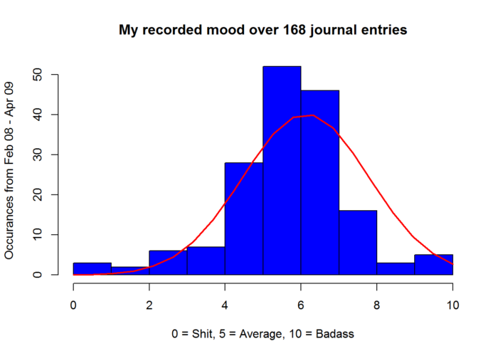
## 1   1 168 6.12 1.67      6    6.22 1.48   0  10    10 -0.8     2.48 0.13

moodhist <- hist(mood, col="blue", xlab="0 = Shit, 5 = Average, 10 = Badass", 
ylab = "Occurances from Feb 08 - Apr 09", main = "My recorded mood over 168 journal entries")
xfit<-seq(min(mood), max(mood),length=20)
yfit<-dnorm(xfit,mean=mean(mood),sd=sd(mood)) 
yfit <- yfit*diff(moodhist$mids[1:2])*length(mood) 
lines(xfit, yfit, col="red", lwd=2) 

moodhist <- hist(mood, breaks = 2, col="blue", xlab="Highlighting: 0-4 = Less than average mood", 
ylab = "Occurances from Feb 08 - Apr 09", main = "My recorded mood over 168 journal entries")
xfit<-seq(min(mood), max(mood),length=10)
yfit<-dnorm(xfit,mean=mean(mood),sd=sd(mood)) 
yfit <- yfit*diff(moodhist$mids[1:2])*length(mood) 
lines(xfit, yfit, col="red", lwd=2) 

ggplot() + aes(mood)+ geom_histogram(binwidth=1,breaks=seq (0, 10, by = 1), colour="black", 
aes(fill= ..count.., y=..density.. )) + scale_fill_gradient("Observation Counts",
low = "red", high = "green") + xlim (c(0,10)) + xlab("Mood when journaling skews heavily positive
between 6 and 10") + geom_density( col = 1, size = 1)

plot (mood,type = "b", pch = 20, lty = 3, xlab = "Mood over time highlighing one standard deviation", 
ylab = "Scale: 0-Unhealthy, 5-Normal, 10-Badass")
dmood <- describe(mood)
moodmean <- dmood[3]
abline (h=moodmean, col="green")
moodsd <- dmood[4]
moodusd <- moodmean + moodsd
abline(h=moodusd, col="red")
moodlsd <- moodmean - moodsd
abline (h=moodlsd, col="red")

dfeb08 = seq(as.Date("2008/2/1"), as.Date("2008/2/13"), "days")
dmar08 = seq(as.Date("2008/3/1"), as.Date("2008/3/13"), "days")
dapr08 = seq(as.Date("2008/4/1"), as.Date("2008/4/2"), "days")
dmay08 = seq(as.Date("2008/5/1"), as.Date("2008/5/1"), "days")
djun08 = seq(as.Date("2008/6/1"), as.Date("2008/6/2"), "days")
djul08 = seq(as.Date("2008/7/1"), as.Date("2008/7/12"), "days")
daug08 = seq(as.Date("2008/8/1"), as.Date("2008/8/7"), "days")
dsept08 = seq(as.Date("2008/9/1"), as.Date("2008/9/7"), "days")
doct08 = seq(as.Date("2008/10/1"), as.Date("2008/10/16"), "days")
dnov08 = seq(as.Date("2008/11/1"), as.Date("2008/11/9"), "days")
ddec08 = seq(as.Date("2008/12/1"), as.Date("2008/12/16"), "days")
djan09 = seq(as.Date("2009/1/1"), as.Date("2009/1/23"), "days")
dfeb09 = seq(as.Date("2009/2/1"), as.Date("2009/2/19"), "days")
dmar09 = seq(as.Date("2009/3/1"), as.Date("2009/3/20"), "days")
dapr09 = seq(as.Date("2009/4/1"), as.Date("2009/4/9"), "days")

feb08.mood = zoo(x=feb08, order.by = dfeb08)
mar08.mood = zoo(x=mar08, order.by = dmar08)
apr08.mood = zoo(x=apr08, order.by = dapr08)
may08.mood = zoo(x=may08, order.by = dmay08)
jun08.mood = zoo(x=jun08, order.by = djun08)
jul08.mood = zoo(x=jul08, order.by = djul08)
aug08.mood = zoo(x=aug08, order.by = daug08)
sept08.mood = zoo(x=sept08, order.by = dsept08)
oct08.mood = zoo(x=oct08, order.by = doct08)
nov08.mood = zoo(x=nov08, order.by = dnov08)
dec08.mood = zoo(x=dec08, order.by = ddec08)
jan09.mood = zoo(x=jan09, order.by = djan09)
feb09.mood = zoo(x=feb09, order.by = dfeb09)
mar09.mood = zoo(x=mar09, order.by = dmar09)
apr09.mood = zoo(x=apr09, order.by = dapr09)

finalmood = cbind(feb08.mood,mar08.mood, apr08.mood, may08.mood, jun08.mood, 
jul08.mood, aug08.mood, sept08.mood, oct08.mood, nov08.mood, dec08.mood, jan09.mood,
feb09.mood, mar09.mood, apr09.mood)

moodlist <- list(feb08.mood,mar08.mood, apr08.mood, may08.mood, jun08.mood, jul08.mood, 
aug08.mood, sept08.mood, oct08.mood, nov08.mood, dec08.mood, jan09.mood, feb09.mood, mar09.mood, apr09.mood) 
moodlength <- lapply (moodlist, length)
moodcolor <- c()
for (i in 1:length(moodlength)) {
  if (moodlength[[i]] <= 10) {
    color <- ("red")
  } else {
    color <- ("blue")
  }
  moodcolor <- append(moodcolor,color)
}

plot (finalmood, type='b', pch=20, plot.type = "single", col=moodcolor, 
xlab=("Journal Entries Feb08 - Apr09"), ylab = "Scale: 0-Unhealthy, 5-Normal, 10-Badass") 
legend (x="bottomright", legend = c("Blue >= 10", "Red <= 10"), col=c("blue","red"), lty = 1:1)
mtext("Feb08  Mar   Apr  May   Jun   Jul  Aug  Sep  Oct  Nov  Dec  Jan  Feb  Mar  Apr", 
side = 1, line = 2, adj=0, cex =.80)